Use AMICA in a Scikit-Learn Pipeline¶

We’ll use AMICA as a preprocessing step in a scikit-learn pipeline to perform digit classification on the MNIST dataset.

import numpy as np
import matplotlib.pyplot as plt

from sklearn.datasets import fetch_openml
from sklearn.model_selection import train_test_split
from sklearn.preprocessing import StandardScaler
from sklearn.pipeline import Pipeline
from sklearn.linear_model import LogisticRegression
from sklearn.metrics import classification_report

from amica import AMICA

Load & split dataset

Download MNIST (70k samples, 28×28 flattened)

X, y = fetch_openml("mnist_784", version=1, return_X_y=True, as_frame=False)

# Just take digits 0-3 to speed up computation
mask = np.isin(y, ["0", "1", "2", "3"])
X = X[mask].copy()
y = y[mask].copy().astype(int)

# Train/test split: 60k / 10k
X_train, X_test, y_train, y_test = train_test_split(
    X, y, test_size=1/7.0, shuffle=True, random_state=0
)

Build scikit-learn pipeline with AMICA¶

pipe = Pipeline([
    ("center", StandardScaler(with_std=False)),  # remove global brightness bias
    ("amica", AMICA(n_components=60, max_iter=200, tol=.0001, random_state=0)),
    ("scale_components", StandardScaler()),      # optional but helps LR
    ("logreg", LogisticRegression(
        max_iter=2000,
        n_jobs=-1
    )),
])

Fit¶

pipe.fit(X_train, y_train)

/home/circleci/project/amica-python/src/amica/linalg.py:333: RuntimeWarning: invalid value encountered in sqrt
  Winv = (eigvecs * np.sqrt(eigvals)) @ eigvecs.T  # Inverse of the whitening matrix

/home/circleci/project/amica-python/.venv/lib/python3.11/site-packages/sklearn/linear_model/_logistic.py:1184: FutureWarning: 'n_jobs' has no effect since 1.8 and will be removed in 1.10. You provided 'n_jobs=-1', please leave it unspecified.
  warnings.warn(msg, category=FutureWarning)

Pipeline(steps=[('center', StandardScaler(with_std=False)),
                ('amica',
                 AMICA(max_iter=200, n_components=60, random_state=0,
                       tol=0.0001)),
                ('scale_components', StandardScaler()),
                ('logreg', LogisticRegression(max_iter=2000, n_jobs=-1))])

In a Jupyter environment, please rerun this cell to show the HTML representation or trust the notebook.
On GitHub, the HTML representation is unable to render, please try loading this page with nbviewer.org.

Evaluate¶

y_pred = pipe.predict(X_test)

print(classification_report(
    y_test, y_pred, target_names=[str(i) for i in range(4)]
))

print(f"Accuracy: {pipe.score(X_test, y_test):.4f}")

              precision    recall  f1-score   support

           0       0.98      0.99      0.98       951
           1       0.98      0.99      0.98      1135
           2       0.96      0.94      0.95       988
           3       0.97      0.96      0.97      1057

    accuracy                           0.97      4131
   macro avg       0.97      0.97      0.97      4131
weighted avg       0.97      0.97      0.97      4131

Accuracy: 0.9717

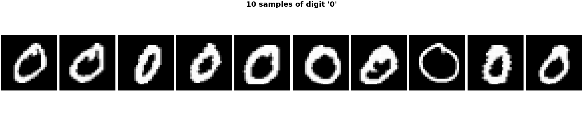
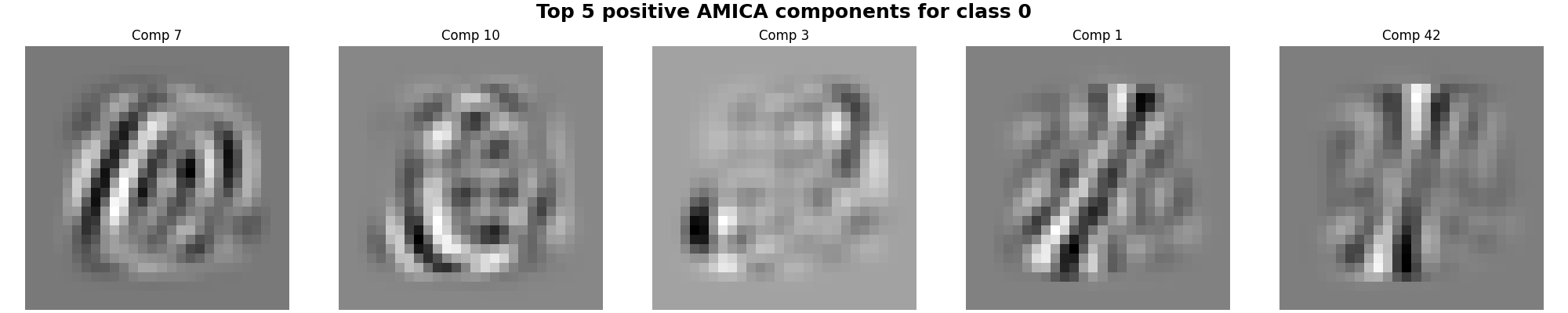
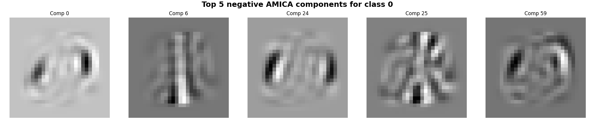
Important features for the 0 digit¶

We can select the most important ICA features for the 0 class (with negative and positive weights) and display their associate ICA sources.

Helper¶

def imshow_row(images, titles=None, figsize=(20, 4), suptitle=None, cmap="gray"):
    fig, axes = plt.subplots(1, len(images), figsize=figsize, constrained_layout=True)
    if suptitle:
        fig.suptitle(suptitle, fontsize=18, fontweight="bold")
    for i, ax in enumerate(axes):
        ax.imshow(images[i].reshape(28, 28), cmap=cmap)
        ax.axis("off")
        if titles is not None:
            ax.set_title(titles[i])
    return fig

Show sample digits of class 0¶

zeros = X[y == 0][:10]

imshow_row(
    zeros,
    suptitle="10 samples of digit '0'"
)
plt.show()

Top positive / negative logistic weights¶

logreg = pipe.named_steps["logreg"]
amica = pipe.named_steps["amica"]

coef = logreg.coef_[0]
sorted_idx = np.argsort(coef)

top_pos = sorted_idx[-5:][::-1]
top_neg = sorted_idx[:5]

imshow_row(
    amica.components_[top_pos],
    titles=[f"Comp {i}" for i in top_pos],
    suptitle="Top 5 positive AMICA components for class 0"
)
plt.show()

Top 5 positive AMICA components for class 0, Comp 19, Comp 30, Comp 9, Comp 3, Comp 39

imshow_row(
    amica.components_[top_neg],
    titles=[f"Comp {i}" for i in top_neg],
    suptitle="Top 5 negative AMICA components for class 0"
)
plt.show()

Top 5 negative AMICA components for class 0, Comp 0, Comp 59, Comp 16, Comp 22, Comp 57

Total running time of the script: (1 minutes 49.319 seconds)

Gallery generated by Sphinx-Gallery

	steps steps: list of tuples List of (name of step, estimator) tuples that are to be chained in sequential order. To be compatible with the scikit-learn API, all steps must define `fit`. All non-last steps must also define `transform`. See :ref:`Combining Estimators ` for more details.	[('center', ...), ('amica', ...), ...]
	transform_input transform_input: list of str, default=None The names of the :term:`metadata` parameters that should be transformed by the pipeline before passing it to the step consuming it. This enables transforming some input arguments to ``fit`` (other than ``X``) to be transformed by the steps of the pipeline up to the step which requires them. Requirement is defined via :ref:`metadata routing `. For instance, this can be used to pass a validation set through the pipeline. You can only set this if metadata routing is enabled, which you can enable using ``sklearn.set_config(enable_metadata_routing=True)``. .. versionadded:: 1.6	None
	memory memory: str or object with the joblib.Memory interface, default=None Used to cache the fitted transformers of the pipeline. The last step will never be cached, even if it is a transformer. By default, no caching is performed. If a string is given, it is the path to the caching directory. Enabling caching triggers a clone of the transformers before fitting. Therefore, the transformer instance given to the pipeline cannot be inspected directly. Use the attribute ``named_steps`` or ``steps`` to inspect estimators within the pipeline. Caching the transformers is advantageous when fitting is time consuming. See :ref:`sphx_glr_auto_examples_neighbors_plot_caching_nearest_neighbors.py` for an example on how to enable caching.	None
	verbose verbose: bool, default=False If True, the time elapsed while fitting each step will be printed as it is completed.	False

	n_components	60
	n_mixtures	3
	batch_size	None
	device	'cpu'
	n_models	1
	mean_center	True
	whiten	'zca'
	max_iter	200
	tol	0.0001
	lrate	0.05
	pdftype	0
	do_newton	True
	newt_start	50
	newtrate	1.0
	w_init	None
	sbeta_init	None
	mu_init	None
	random_state	0
	verbose	1

	penalty penalty: {'l1', 'l2', 'elasticnet', None}, default='l2' Specify the norm of the penalty: - `None`: no penalty is added; - `'l2'`: add a L2 penalty term and it is the default choice; - `'l1'`: add a L1 penalty term; - `'elasticnet'`: both L1 and L2 penalty terms are added. .. warning:: Some penalties may not work with some solvers. See the parameter `solver` below, to know the compatibility between the penalty and solver. .. versionadded:: 0.19 l1 penalty with SAGA solver (allowing 'multinomial' + L1) .. deprecated:: 1.8 `penalty` was deprecated in version 1.8 and will be removed in 1.10. Use `l1_ratio` instead. `l1_ratio=0` for `penalty='l2'`, `l1_ratio=1` for `penalty='l1'` and `l1_ratio` set to any float between 0 and 1 for `'penalty='elasticnet'`.	'deprecated'
	C C: float, default=1.0 Inverse of regularization strength; must be a positive float. Like in support vector machines, smaller values specify stronger regularization. `C=np.inf` results in unpenalized logistic regression. For a visual example on the effect of tuning the `C` parameter with an L1 penalty, see: :ref:`sphx_glr_auto_examples_linear_model_plot_logistic_path.py`.	1.0
	l1_ratio l1_ratio: float, default=0.0 The Elastic-Net mixing parameter, with `0 <= l1_ratio <= 1`. Setting `l1_ratio=1` gives a pure L1-penalty, setting `l1_ratio=0` a pure L2-penalty. Any value between 0 and 1 gives an Elastic-Net penalty of the form `l1_ratio * L1 + (1 - l1_ratio) * L2`. .. warning:: Certain values of `l1_ratio`, i.e. some penalties, may not work with some solvers. See the parameter `solver` below, to know the compatibility between the penalty and solver. .. versionchanged:: 1.8 Default value changed from None to 0.0. .. deprecated:: 1.8 `None` is deprecated and will be removed in version 1.10. Always use `l1_ratio` to specify the penalty type.	0.0
	dual dual: bool, default=False Dual (constrained) or primal (regularized, see also :ref:`this equation `) formulation. Dual formulation is only implemented for l2 penalty with liblinear solver. Prefer `dual=False` when n_samples > n_features.	False
	tol tol: float, default=1e-4 Tolerance for stopping criteria.	0.0001
	fit_intercept fit_intercept: bool, default=True Specifies if a constant (a.k.a. bias or intercept) should be added to the decision function.	True
	intercept_scaling intercept_scaling: float, default=1 Useful only when the solver `liblinear` is used and `self.fit_intercept` is set to `True`. In this case, `x` becomes `[x, self.intercept_scaling]`, i.e. a "synthetic" feature with constant value equal to `intercept_scaling` is appended to the instance vector. The intercept becomes ``intercept_scaling * synthetic_feature_weight``. .. note:: The synthetic feature weight is subject to L1 or L2 regularization as all other features. To lessen the effect of regularization on synthetic feature weight (and therefore on the intercept) `intercept_scaling` has to be increased.	1
	class_weight class_weight: dict or 'balanced', default=None Weights associated with classes in the form ``{class_label: weight}``. If not given, all classes are supposed to have weight one. The "balanced" mode uses the values of y to automatically adjust weights inversely proportional to class frequencies in the input data as ``n_samples / (n_classes * np.bincount(y))``. Note that these weights will be multiplied with sample_weight (passed through the fit method) if sample_weight is specified. .. versionadded:: 0.17 class_weight='balanced'	None
	random_state random_state: int, RandomState instance, default=None Used when ``solver`` == 'sag', 'saga' or 'liblinear' to shuffle the data. See :term:`Glossary ` for details.	None
	solver solver: {'lbfgs', 'liblinear', 'newton-cg', 'newton-cholesky', 'sag', 'saga'}, default='lbfgs' Algorithm to use in the optimization problem. Default is 'lbfgs'. To choose a solver, you might want to consider the following aspects: - 'lbfgs' is a good default solver because it works reasonably well for a wide class of problems. - For :term:`multiclass` problems (`n_classes >= 3`), all solvers except 'liblinear' minimize the full multinomial loss, 'liblinear' will raise an error. - 'newton-cholesky' is a good choice for `n_samples` >> `n_features * n_classes`, especially with one-hot encoded categorical features with rare categories. Be aware that the memory usage of this solver has a quadratic dependency on `n_features * n_classes` because it explicitly computes the full Hessian matrix. - For small datasets, 'liblinear' is a good choice, whereas 'sag' and 'saga' are faster for large ones; - 'liblinear' can only handle binary classification by default. To apply a one-versus-rest scheme for the multiclass setting one can wrap it with the :class:`~sklearn.multiclass.OneVsRestClassifier`. .. warning:: The choice of the algorithm depends on the penalty chosen (`l1_ratio=0` for L2-penalty, `l1_ratio=1` for L1-penalty and `0 < l1_ratio < 1` for Elastic-Net) and on (multinomial) multiclass support: ================= ======================== ====================== solver l1_ratio multinomial multiclass ================= ======================== ====================== 'lbfgs' l1_ratio=0 yes 'liblinear' l1_ratio=1 or l1_ratio=0 no 'newton-cg' l1_ratio=0 yes 'newton-cholesky' l1_ratio=0 yes 'sag' l1_ratio=0 yes 'saga' 0<=l1_ratio<=1 yes ================= ======================== ====================== .. note:: 'sag' and 'saga' fast convergence is only guaranteed on features with approximately the same scale. You can preprocess the data with a scaler from :mod:`sklearn.preprocessing`. .. seealso:: Refer to the :ref:`User Guide ` for more information regarding :class:`LogisticRegression` and more specifically the :ref:`Table ` summarizing solver/penalty supports. .. versionadded:: 0.17 Stochastic Average Gradient (SAG) descent solver. Multinomial support in version 0.18. .. versionadded:: 0.19 SAGA solver. .. versionchanged:: 0.22 The default solver changed from 'liblinear' to 'lbfgs' in 0.22. .. versionadded:: 1.2 newton-cholesky solver. Multinomial support in version 1.6.	'lbfgs'
	max_iter max_iter: int, default=100 Maximum number of iterations taken for the solvers to converge.	2000
	verbose verbose: int, default=0 For the liblinear and lbfgs solvers set verbose to any positive number for verbosity.	0
	warm_start warm_start: bool, default=False When set to True, reuse the solution of the previous call to fit as initialization, otherwise, just erase the previous solution. Useless for liblinear solver. See :term:`the Glossary `. .. versionadded:: 0.17 warm_start to support lbfgs, newton-cg, sag, saga solvers.	False
	n_jobs n_jobs: int, default=None Does not have any effect. .. deprecated:: 1.8 `n_jobs` is deprecated in version 1.8 and will be removed in 1.10.	-1

	copy copy: bool, default=True If False, try to avoid a copy and do inplace scaling instead. This is not guaranteed to always work inplace; e.g. if the data is not a NumPy array or scipy.sparse CSR matrix, a copy may still be returned.	True
	with_mean with_mean: bool, default=True If True, center the data before scaling. This does not work (and will raise an exception) when attempted on sparse matrices, because centering them entails building a dense matrix which in common use cases is likely to be too large to fit in memory.	True
	with_std with_std: bool, default=True If True, scale the data to unit variance (or equivalently, unit standard deviation).	False