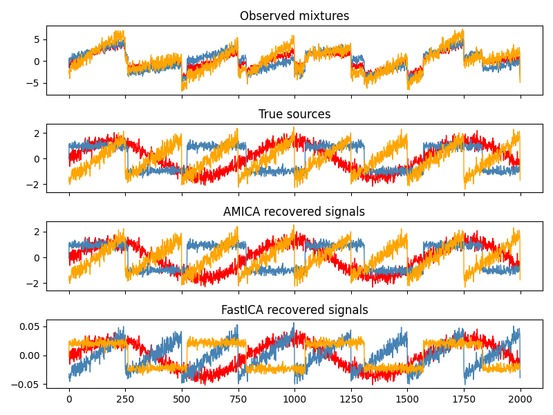
Blind Source Separation with AMICA & FastICA

An example of estimating sources from noisy mixtures.

ICA separates independent sources given only mixed microphone recordings. Imagine three instruments playing simultaneously and three microphones recording the mixtures. ICA recovers the instrument tracks because the sources are non-Gaussian. PCA, by contrast, fails in this setting.

Note

This example is adapted from the Scikit-Learn documentation.

Generate sample data

import numpy as np
from scipy import signal

rng = np.random.default_rng(0)
n_samples = 2000
time = np.linspace(0, 8, n_samples)

s1 = np.sin(2 * time)                     # Sinusoidal
s2 = np.sign(np.sin(3 * time))            # Square wave
s3 = signal.sawtooth(2 * np.pi * time)    # Sawtooth

S = np.c_[s1, s2, s3]
S += 0.2 * rng.standard_normal(S.shape)   # Add noise
S /= S.std(axis=0)                        # Standardize

A = np.array([[1, 1, 1],
              [0.5, 2, 1.0],
              [1.5, 1.0, 2.0]])           # Mixing matrix

X = S @ A.T                               # Observed mixtures

Run AMICA and FastICA

from amica import AMICA
from sklearn.decomposition import FastICA

models = {}
labels = {}

# AMICA
# We instantiate amica.AMICA and call fit..
ica = AMICA(n_components=3, whiten="zca", random_state=0)
models["AMICA"] = ica.fit_transform(X)
labels["AMICA"] = "AMICA recovered signals"

We can prove that the ICA model applies by reverting the unmixing.

X_rec = models["AMICA"] @ ica.mixing_.T + ica.mean_
np.testing.assert_allclose(X, X_rec)

# FastICA
fastica = FastICA(n_components=3, whiten="arbitrary-variance", random_state=0)
models["FastICA"] = fastica.fit_transform(X)
labels["FastICA"] = "FastICA recovered signals"

Plot results

import matplotlib.pyplot as plt

# Merge dictionaries into one mapping title -> data
to_plot = {
    "Observed mixtures": X,
    "True sources": S,
}
to_plot.update({ labels[k]: v for k, v in models.items() })

colors = ["red", "steelblue", "orange"]

fig, axes = plt.subplots(len(to_plot), 1, figsize=(8, 6), sharex=True)
for ax, (title, model) in zip(axes, to_plot.items()):
    ax.set_title(title)
    for sig, color in zip(model.T, colors):
        ax.plot(sig, color=color, lw=1)

plt.tight_layout()
plt.show()