Note
Go to the end to download the full example code.
Accelerate coordinate ascent updates for linear regression
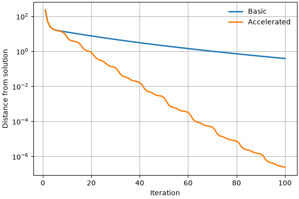
This example compares ordinary coordinate ascent with DAAREM acceleration for a ridge regression model. It is the Python version of this corresponding R daarem demo.
Set up the simulation
import time
import warnings

import matplotlib.pyplot as plt
import numpy as np
from pydaarem import daarem

rng = np.random.default_rng(0)
n = 200
p = 500
na = 10
se = 4
s0 = 1 / se


def simulate_predictors_decaying_corr(n, p, s=0.5, rng=None):
    """Draw predictors with correlations that decay by distance."""
    S = s ** abs(np.subtract.outer(np.arange(1, p + 1), np.arange(1, p + 1)))
    if rng is None:
        rng = np.random.default_rng()
    return rng.multivariate_normal(np.zeros(p), S, n)


def ridge_objective(X, y, b, s0):
    """Compute the log-posterior objective up to a constant."""
    residual = y - X @ b
    return -(np.linalg.norm(residual) ** 2 + np.linalg.norm(b) ** 2 / s0)


def ridge_update(X, y, b, s0):
    """Apply one coordinate ascent update for each coefficient."""
    p = len(b)
    d = np.sum(X**2, axis=0)
    xy = y @ X
    xb = X @ b

    b = b.copy()

    for i in range(p):
        b0 = b[i]
        b[i] = (xy[i] + d[i] * b[i] - xb @ X[:, i]) / (d[i] + 1 / s0)
        xb += (b[i] - b0) * X[:, i]

    return b


def ridge(X, y, b0, s0, numiter=100):
    """Fit ridge regression using coordinate ascent updates."""
    b = np.asarray(b0).copy()
    value = np.zeros(numiter)

    for iteration in range(numiter):
        b = ridge_update(X, y, b, s0)
        value[iteration] = ridge_objective(X, y, b, s0)

    return {"b": b, "value": value}


def daarridge(X, y, b0, s0, numiter=100, order=10):
    """Fit ridge regression using DAAREM-accelerated coordinate ascent."""

    nupd = 0
    nobj = 0

    # Objective function passed to DAAREM.
    def objective(b, X, y, s0):
        nonlocal nobj
        nobj += 1
        return ridge_objective(X, y, b, s0)

    # Fixed-point function passed to DAAREM.
    def update(b, X, y, s0):
        nonlocal nupd
        nupd += 1
        return ridge_update(X, y, b, s0)

    # Run DAAREM.
    with warnings.catch_warnings():
        warnings.simplefilter("ignore")
        out = daarem(
            b0,
            update,
            objective,
            X,
            y,
            s0,
            control={
                "maxiter": numiter,
                "order": order,
                "tol": 0,
                "mon_tol": 0,
                "kappa": 20,
                "alpha": 1.2,
            },
        )

    # Return coefficient estimates, objective history, and evaluation counts.
    return {
        "b": out["par"],
        "value": out["objfn_track"][1:],
        "nupd": nupd,
        "nobj": nobj,
    }
Simulate a data set
Run ordinary coordinate ascent
Computation took 0.21 seconds.
Objective value at solution is -18.327340983670.
Run accelerated coordinate ascent
Computation took 0.28 seconds.
Objective value at solution is -17.942947890329.
Plot improvement in the solution
# The exact ridge solution provides a reference for the distance plot.
bhat = np.linalg.solve(X.T @ X + np.eye(p) / s0, X.T @ y)
f = ridge_objective(X, y, bhat, s0)

iterations = np.arange(1, len(fit1["value"]) + 1)
fig, ax = plt.subplots(figsize=(6, 4), layout="constrained")
ax.plot(iterations, f - fit1["value"], linewidth=2, label="Basic")
ax.plot(iterations, f - fit2["value"], linewidth=2, label="Accelerated")
ax.set_yscale("log")
ax.set_xlabel("Iteration")
ax.set_ylabel("Distance from solution")
ax.grid(True, which="major", linewidth=0.8)
ax.set_axisbelow(True)
ax.legend(frameon=False)
plt.show()
Total running time of the script: (0 minutes 0.727 seconds)